The short version: if Monday closes down, buy QQQ at the close and sell at the first close above the previous day's high. From 2003 to June 2026 that produced 410 trades with a 77% win rate overall — and in the out-of-sample window (2019–2026) it returned 13.7% per year with an 81.4% win rate and a max drawdown under 10%, while in the market just 18% of the time.
The rules
The setup is almost embarrassingly simple — two rules, no indicators, nothing to optimize:
Turnaround Tuesday — complete rules
- Entry: if Monday closes below the previous trading day's close, buy at Monday's close.
- Exit: sell at the first daily close above the previous day's high.
That's the entire strategy. It's either in the market waiting for the exit condition, or flat waiting for the next weak Monday. The average trade lasts about three days, and the entry fires on roughly one in three Mondays.
The logic: markets tend to overreact going into the week. Weekend headlines, anxiety, and Monday selling often push prices below what the actual news flow justifies — and the snap-back concentrates early in the week. The exit rule lets the bounce run until buyers have demonstrably taken control (a close above the prior day's high), rather than cutting the trade at an arbitrary time.
Why Tuesday, specifically?
This isn't a story we made up to fit the backtest — the day-of-week asymmetry is visible in raw index data. Here's the cumulative return of SPY split by weekday since 1993, with no strategy applied at all:
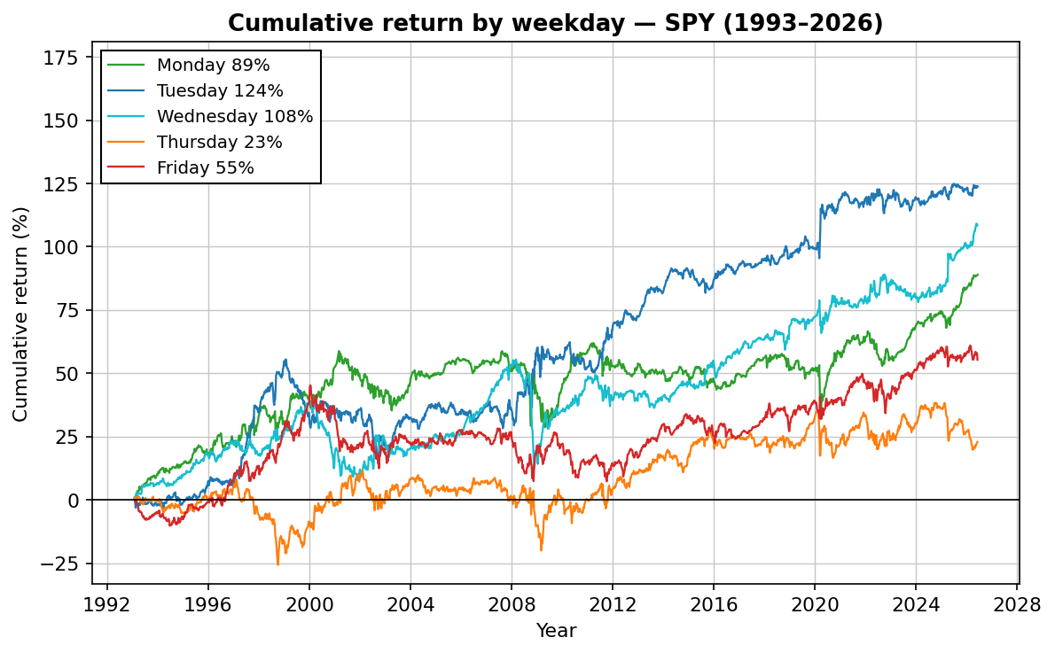
Tuesday is the strongest day of the week over 33 years of data (+124% cumulative, against +23% for Thursday). But the more interesting cut is conditional: Tuesdays that follow a down Monday outperform all Tuesdays combined — even though they're only 40% of them:
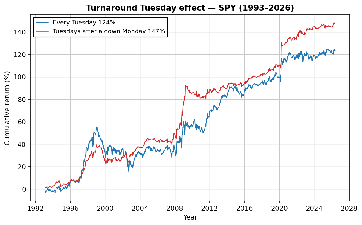
That's the Turnaround Tuesday effect in its rawest form: 683 days carrying more return than all 1,725 Tuesdays together. The strategy below is just a disciplined way of harvesting it — with a defined entry, a defined exit, and no judgment calls.
How we tested it
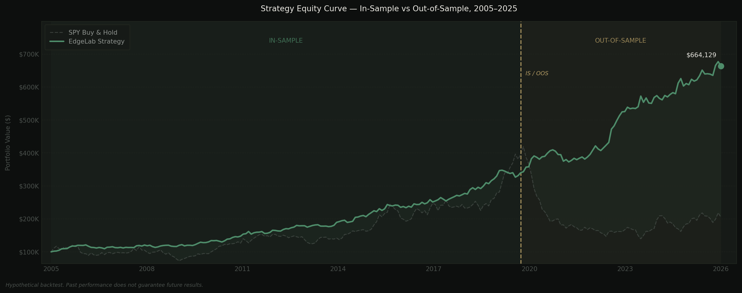
Most strategy writeups show a single equity curve: all the data, parameters already dialled in, presented as proof. That's not a test — it's a description of the past dressed up as a prediction.
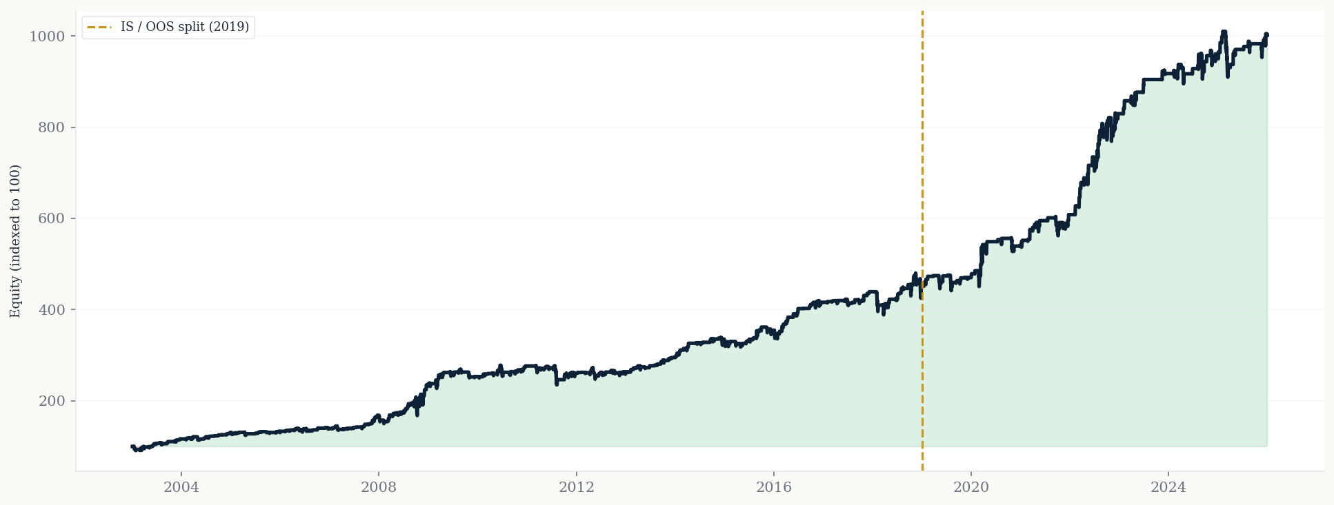
Every strategy at EdgeLab goes through a strict in-sample / out-of-sample split. The data is divided once, up front, and the out-of-sample window stays locked during development. Whatever comes out of that held-back data is the result. No re-tuning afterwards.
- In-sample: January 2003 – December 2018 (16 years, 292 trades). Used to verify the concept and check sensitivity.
- Out-of-sample: January 2019 – June 2026 (7.5 years, 118 trades). Never touched during development.
All results include a 0.05% round-trip commission. Data is dividend-adjusted daily QQQ and SPY.
The numbers
| Metric | In-sample (2003–2018) | Out-of-sample (2019–2026) |
|---|---|---|
| CAGR | 10.9% | 13.7% |
| Sharpe ratio | 0.89 | 1.17 |
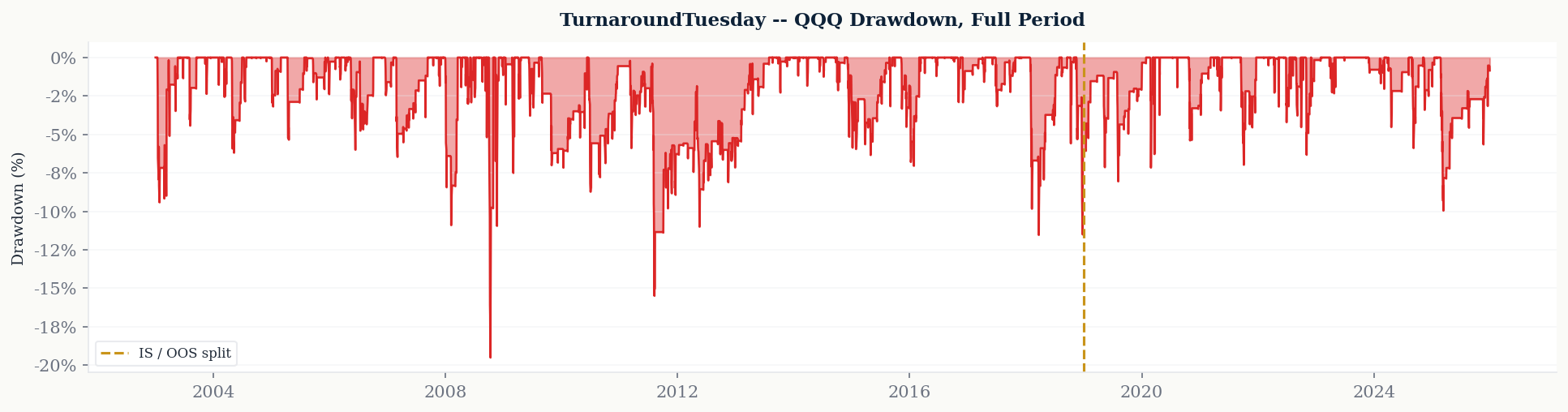
| Max drawdown | -19.5% | -9.9% |
| Win rate | 75.7% | 81.4% |
| Profit factor | 2.39 | 3.21 |
| Trades | 292 | 118 |
| Time in market | 25.4% | 18.1% |
The out-of-sample window beats the development period on every meaningful metric: higher Sharpe, half the drawdown, better win rate. When a strategy's worst period is its development data, overfitting becomes an unlikely explanation — though OOS outperformance deserves its own scrutiny, which we get to below.
410 trades in 23½ years — and 77% of that time the strategy sat in cash, waiting.
Same rules, different market: SPY
A strategy that only works on one instrument is usually an artefact of that instrument's history. So we ran the identical rules — zero changes — on SPY as a validation market:
| Out-of-sample (2019–2026) | QQQ (primary) | SPY (validation) |
|---|---|---|
| CAGR | 13.7% | 12.6% |
| Sharpe ratio | 1.17 | 1.23 |
| Max drawdown | -9.9% | -11.3% |
| Win rate | 81.4% | 79.7% |
| Trades | 118 | 128 |
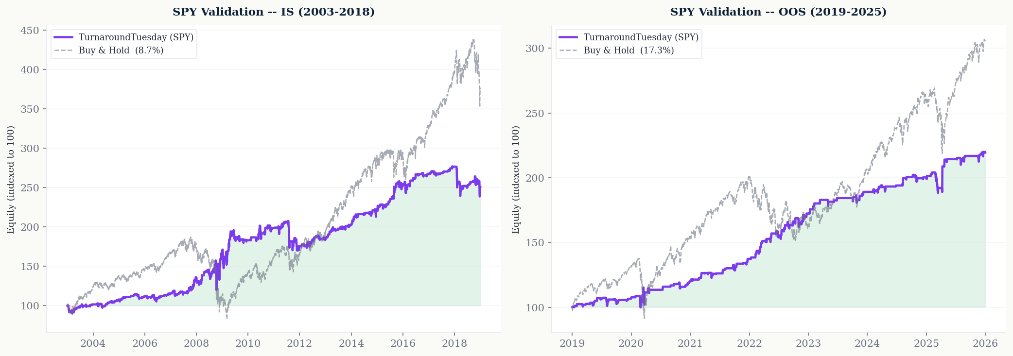
This is what validation should look like: not a tweaked variation that also works, but independent confirmation on a different index. Win rates within two percentage points, Sharpe ratios within 0.06. The edge is a broad large-cap index effect, not a QQQ quirk.
What to watch for
An honest writeup has to flag the uncomfortable parts too. Three things we keep an eye on:
1. OOS is better than IS. Usually it's the other way around. Part of the explanation is regime: 2019–2026 contained several violent, mean-reversion-rich episodes — the COVID crash, the 2022 rate shock, the 2025 tariff selloff. Conditions like that are unusually good for a strategy that buys panic Mondays. In a long, quiet, grinding bull market the strategy fires less often and earns less. When we re-ran the test in June 2026 to extend the out-of-sample window, the win rate had actually ticked up — pleasant, but we treat it as the favorable end of the range, not the expectation.
2. Trade count is modest. 118 OOS trades is a reasonable statistical base, but at ~16 trades per year, individual years vary a lot. 2022 still worked, by a thinner margin. A flat or losing year shouldn't surprise anyone — and shouldn't trigger re-optimization.
3. The exit has no stop. The strategy holds until a close above the prior day's high. In a sustained decline that means sitting through several down days — the -19.5% drawdown in 2008 is what that looks like in practice. Position sizing, not a stop loss, is the risk control here.
How to trade it
- Monday, just before the close: if QQQ (or SPY) is trading below the previous close, enter long at or near the close.
- Each following day at the close: if the close is above yesterday's high, exit. Otherwise hold.
- Position size so that a ~20% strategy drawdown is survivable for you. Given the profile, 10–20% of a portfolio is the range we'd consider.
- No overrides. The edge comes from taking every signal. The moment you start skipping "scary" Mondays, you're trading a different — untested — strategy.
Execution is simple enough for a TradingView alert at Monday's close, or a few lines against a broker API. Implementation error is a bigger risk than signal interpretation.
Get the Python backtest for this strategy
The complete, runnable script behind this article — data download (free, via yfinance), backtest engine, stats and charts. Plus our two free strategy reports as PDFs.
No spam. Unsubscribe anytime.
Done — here are your downloads:
- turnaround-tuesday.py — the full backtest script
- Your two free strategy reports (PDF) →
FAQ
What is the Turnaround Tuesday strategy?
Turnaround Tuesday is a mean-reversion strategy for stock indices: if Monday closes below the previous close, buy at Monday's close. Sell at the first close above the previous day's high. The typical trade lasts two to three days, and the strategy is in the market less than a quarter of the time.
Does Turnaround Tuesday still work in 2026?
In our out-of-sample test on QQQ from January 2019 to June 2026 — data not used during development — the strategy returned 13.7% annually with an 81.4% win rate and a maximum drawdown of -9.9%. The recent period has been unusually favorable for mean reversion, so we treat those numbers as the optimistic end of the range.
Which markets does it work on?
We tested QQQ as the primary instrument and validated the identical rules on SPY, which produced nearly identical results (out-of-sample Sharpe 1.23 vs 1.17). It's a large-cap US index effect; we haven't validated it on small caps, individual stocks or other asset classes — and on IWM, related mean-reversion setups have historically been much weaker.
How often does the strategy trade?
The entry triggers on roughly one in three Mondays — about 16–18 trades per year. Across 23½ years it took 410 trades and sat in cash 77% of the time.

Robin Eriksson
Founder of EdgeLab. Five years of discretionary losses taught me to test everything — now I publish the strategies that survive. About me →
Related: Why your backtest passes — and your live account doesn't · Buying the dip in QQQ: 23 years of evidence · How many trading strategies do you need?