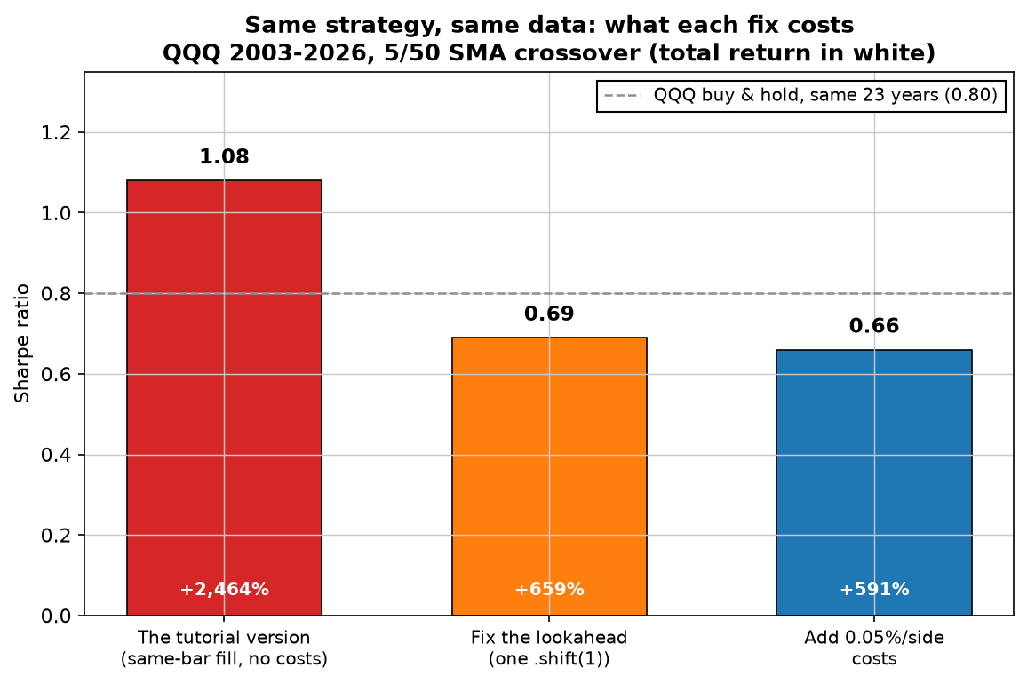
The short version: A textbook SMA crossover on QQQ returns +2,464% with a Sharpe of 1.08 over 23 years. Fix the lookahead — one .shift(1) — and it is +659%. Add realistic costs and it is +591%. Then choose the parameters honestly, on the first half of the data only, and the out-of-sample result is a Sharpe of 0.77 against 0.93 for simply owning QQQ. And one honest catch: the tuning step that every tutorial teaches is the one that did the most damage — it scored worse than picking parameters at random.
The tutorial version returns +2,464%, and the code is twelve lines
The strategy is the one every backtesting tutorial uses: a moving-average crossover. Go long when the fast average is above the slow one, sit in cash otherwise. I ran a small grid of window pairs over the full history and kept the best, which is exactly what a tutorial does — fast 5, slow 50.
The version you will find on the internet
import pandas as pd

px = pd.read_csv("QQQ.csv", index_col=0, parse_dates=True)["close"]
px = px.loc["2002-01-01":]                # warm-up for the 50-day window

fast = px.rolling(5).mean()
slow = px.rolling(50).mean()
returns = px.pct_change()

position = (fast > slow).astype(int)
strategy = (position * returns).loc["2003-01-01":]   # <- the bug is here
equity = (1 + strategy.fillna(0)).cumprod()

print(f"Total return: {(equity.iloc[-1] - 1) * 100:,.0f}%")
# Total return: 2,464%
Nothing about that output looks suspicious. The equity curve is smooth, the drawdown is a mild −18.2%, the Sharpe is 1.08. It is the kind of result that makes people open a brokerage account.
It is also impossible.
One line of code is worth 1,805 percentage points
Look at what position * returns actually says. The position on any given day is computed from that day's closing price — the moving averages end on today's close. The return on that same row is also today's move. So the strategy is deciding what to hold today using a number it cannot know until today is over, and then collecting today's move as though it had been holding all along.
The fix is one call. Decide on today's close, trade on tomorrow's.
The same strategy, honest
position = (fast > slow).astype(int).shift(1)   # decide today, trade tomorrow
turnover = position.diff().abs()                  # 1.0 on every switch
strategy = (position * returns - turnover * 0.0005).loc["2003-01-01":]
equity = (1 + strategy.fillna(0)).cumprod()

print(f"Total return: {(equity.iloc[-1] - 1) * 100:,.0f}%")
# Total return: 591%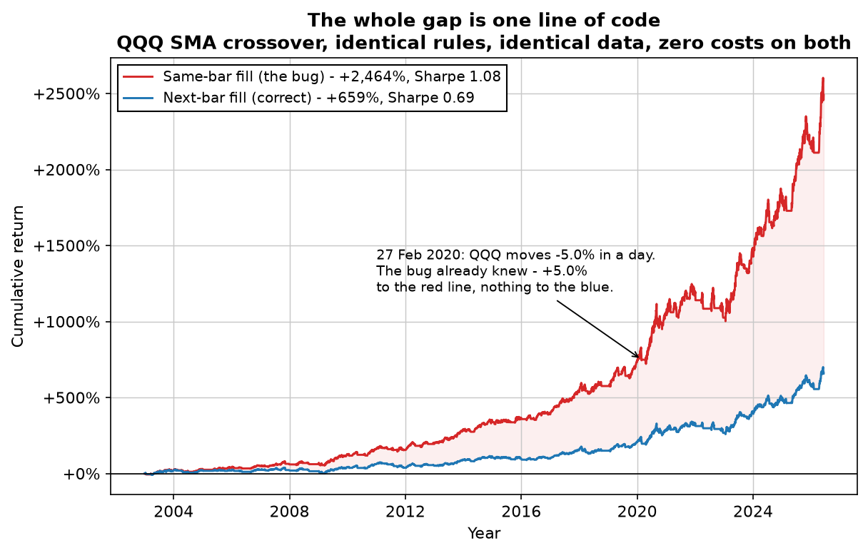
.shift(1). The shaded area is the part of the result that never existed.The annotated day is worth sitting with. On 27 February 2020, QQQ fell 5.0% as the pandemic repriced everything. The buggy version was already flat that day — its moving averages had crossed on that very close, so it "knew". The correct version was still long, because on the previous close the cross had not happened yet. Five percentage points, on one day, from a decision no live account could have made.
That is also why the bug is so hard to spot by eye: it does not produce implausible trades. It produces perfectly plausible trades with slightly impossible timing, and the advantage compounds quietly for two decades.
Costs barely dented it — and that is a warning, not a relief
Adding 0.05% per side — deliberately two to three times what an ETF trade actually costs — took the result from +659% to +591%. In Sharpe terms, 0.69 to 0.66. If you have read that costs destroy backtests, this looks like a counterexample.
It is not. It is a statement about turnover. This strategy changed position 189 times in 23 years, roughly eight times a year. At eight round trips a year, a 0.05% charge is nearly invisible. The same charge on a strategy that trades every day would remove something like 25% a year and turn almost any edge into a loss.
So the honest reading is: cost sensitivity is not a property of your cost assumption, it is a property of your strategy. A slow strategy tolerates sloppy cost modelling. A fast one is defined by it — which is exactly why the cheapest-looking intraday ideas are usually the ones that die first. We have written about that failure mode at length.
Tuning the parameters made the strategy worse
Now the mistake that is hardest to give up, because it feels like diligence. Every tutorial that gets as far as optimisation tells you to search a grid of parameters and keep the best. I did — but I did it twice, so the search could be graded.
First honestly: score all 15 window combinations on 2003–2013 only, pick the winner, then run it on 2014–2026, which it has never seen. Then compare that against what every combination actually did out-of-sample.
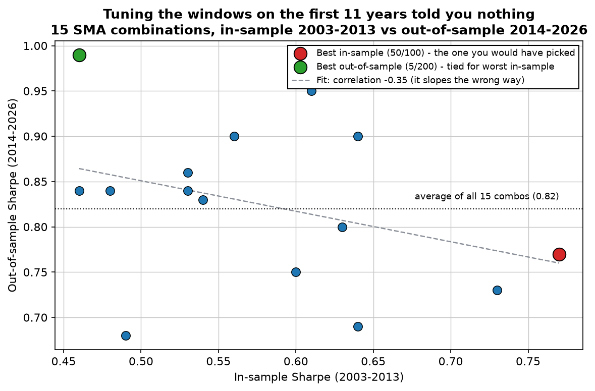
The numbers, plainly. The best in-sample combination (50/100) delivered an out-of-sample Sharpe of 0.77. The average across all 15 combinations was 0.82. Picking the in-sample winner was worse than picking blind. And the best out-of-sample performer, 5/200 at 0.99, was tied for the worst in-sample score on the grid — you would have thrown it away first.
There is a second version of the same trap in the tutorial code above. The 5/50 windows were chosen by searching the whole history. Score that same pair on the first eleven years alone and it ranks 14th out of 15. The "best parameters" were an artefact of the years you let the computer look at.
One caveat I will not dress up: this is 15 combinations on one asset. It is enough to show that in-sample rank did not predict out-of-sample rank here; it is not a general law of markets. The general lesson is smaller and safer — a parameter search buys you far less than it appears to, and you only ever find out by holding data back. Our tripwires for a dying strategy exist for the same reason.
After all four fixes, it loses to simply owning the index
Put the honest version on the out-of-sample years and compare it with the least sophisticated thing available: buying QQQ and doing nothing.
| 2014–2026, net of costs | SMA 50/100 crossover | QQQ buy & hold |
|---|---|---|
| Total return | +347% | +796% |
| CAGR | 12.8% | 19.3% |
| Sharpe | 0.77 | 0.93 |
| Max drawdown | −28.6% | −35.1% |
| Time in market | 80.2% | 100% |
Less return, less risk, and a worse ratio between them. The crossover did do one thing: it cut the worst drawdown by six and a half points while sitting in cash a fifth of the time. That is a real service. It is just not the service the +2,464% seemed to be advertising.
It only wins where buy and hold is weak
The last mistake is testing on one market and one era. QQQ from 2003 is the most flattering chart in modern finance. So I ran the identical rules — same windows, same costs, same out-of-sample window — on four other markets from the frozen data cache.
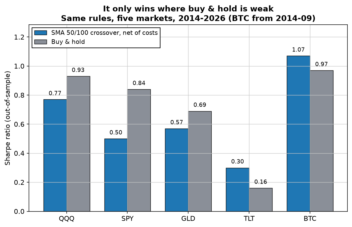
Start with TLT. Long bonds returned 1.3% a year over this period with a Sharpe of 0.16 — a miserable thing to hold. The same crossover that destroyed value on QQQ nearly doubled that Sharpe, to 0.30. On bitcoin it did the same, 0.97 to 1.07, while cutting time in the market to 56%.
That is the useful finding in this whole article, and it has nothing to do with Python. A trend filter is not a return engine — it is drawdown insurance, and like all insurance you pay a premium. When the underlying asset marches upward for twelve years, the premium is all you get. When the asset chops sideways or crashes, the insurance pays. Deciding which of those you are buying is a portfolio question, which is a different article, and it is also why the 200-day moving average survives as a filter and not as a strategy.
The harness, in full
Here is the whole thing — no library, about thirty lines. It takes a price series and returns an honest equity curve. The two switches exist so you can reproduce the bug on purpose and watch what it does to your own strategy.
import numpy as np
import pandas as pd

COMM = 0.0005          # 0.05% per side

def backtest(close, fast, slow, lookahead=False, costs=True):
    signal = close.rolling(fast).mean() > close.rolling(slow).mean()
    position = signal.astype(float)
    if not lookahead:
        position = position.shift(1)         # the line that matters
    position = position.fillna(0.0)

    returns = close.pct_change().fillna(0.0)
    strategy = position * returns
    if costs:
        turnover = position.diff().abs().fillna(position.abs())
        strategy = strategy - turnover * COMM
    return strategy, position

def report(strategy, position):
    equity = (1 + strategy).cumprod()
    years = (strategy.index[-1] - strategy.index[0]).days / 365.25
    bars_per_year = len(strategy) / years    # actual frequency, never 252
    return {
        "total_pct": (equity.iloc[-1] - 1) * 100,
        "cagr_pct": (equity.iloc[-1] ** (1 / years) - 1) * 100,
        "sharpe": strategy.mean() / strategy.std() * np.sqrt(bars_per_year),
        "maxdd_pct": (equity / equity.cummax() - 1).min() * 100,
        "time_in_market_pct": (position > 0).mean() * 100,
    }
Three details in there are doing quiet work. fillna(position.abs()) charges you for the very first entry instead of letting it in free. bars_per_year is measured rather than assumed, so an hourly strategy is not silently annualised as if it were daily. And the flat days stay in the return series as zeros.
That last one is worth a number. On this crossover it barely matters — in the market 69% of the time, deleting the flat rows moves the Sharpe from 0.66 to 0.68. So I built a deliberately rare rule on the same QQQ data, one that holds a position only 4.9% of the time. Its honest Sharpe is 0.67. Delete the flat days and keep annualising with sqrt(252), as almost everyone does, and it reports 3.30 — nearly five times too high, from removing rows that looked like padding. Rare-entry strategies are where this trap lives, and rare-entry strategies are exactly what people sell.
Then hold data back, and check the number you get against what a random parameter choice would have given you. If your tuning cannot beat the average of the grid, it is not tuning. It is decoration.
Lab notes
The first version of the chart above annotated "Oct 2008" as the moment the lookahead bug paid best. That was wrong, and wrong in an instructive way: I had taken the maximum of the cumulative gap inside a 2008–2009 window, and a cumulative gap only grows — so its maximum is always just the last bar of whatever window you searched. It would have printed a confident, meaningless date. Measuring the largest single-day difference instead gave 27 February 2020, which is a real event you can look up.
One more, filed under coincidences that look like proof: the 50/100 windows scored a Sharpe of 0.77 in-sample and 0.77 out-of-sample. Identical to two decimals. If I had run only that pair and stopped there, I would have had a beautiful robustness story — and the other fourteen combinations show it means nothing.
Download a free strategy
Simple and robust — 70% winners across 155 trades over 16 years, net of costs. The free PDF gives you the market, the timeframe and the exact rules in plain English, plus every single trade it has taken.
Instant delivery. One PDF, no spam. Unsubscribe anytime.
FAQ
What is lookahead bias in a Python backtest?
Lookahead bias is using information a trade could not have had at the moment it was placed. In pandas it usually appears as position * returns, where the position was computed from the same bar's close. The fix is one call: shift the position forward by one bar so today's signal earns tomorrow's return. On a QQQ 5/50 SMA crossover over 23 years, that single line is the difference between +2,464% and +659%.
How much do trading costs change a backtest?
It depends entirely on how often the strategy trades. The 5/50 crossover changed position 189 times in 23 years — about eight times a year — so 0.05% per side cost it 68 percentage points of total return, taking it from +659% to +591%. The same charge applied to a strategy that trades daily would remove roughly 25% a year. Costs are not a rounding error; they are a tax on turnover.
Should I optimise my strategy parameters?
Not the way most tutorials teach it. We scored all 15 SMA window combinations on 2003–2013 and then on 2014–2026. The correlation between the two rankings was −0.35: negative. The combination that looked best in-sample delivered an out-of-sample Sharpe of 0.77, below the 0.82 average of simply picking any combination at random. On this grid, tuning was worse than not tuning.
Do I need a backtesting library like backtrader or vectorbt?
Not to answer the question this article asks. Everything here is pandas and numpy in about 30 lines. A library helps with order types, position sizing and multi-asset bookkeeping, but it will not save you from lookahead bias or from optimising on all your data — those are decisions you make, not features you install.

Robin Eriksson
Founder of EdgeLab. Five years of discretionary losses taught me to test everything — now I publish the strategies that survive. About me →
Related: Does the 200-day moving average work? Tested on five assets · Why your backtest passes — and your live account doesn't · Does "sell in May and go away" work? 33 years of SPY, tested