ICT Silver Bullet Strategy Win Rate: 16 Years of Nasdaq Futures (2026)

The short version: over 3,483 trades, our mechanical Silver Bullet won 34.1% of the time with a 2R target and 49.5% with a 1R target. Those numbers sound modest, and they are almost exactly what each payoff needs just to break even. Before costs, the first-gap version earned +0.003R per trade out of sample, which is zero. After a 0.01% round trip it lost -0.096R per trade, and the version that trades with the morning's direction lost -0.142R. Both crossed the failure line I registered before the run: no mechanical edge. And one honest catch: the filter that is supposed to help made it worse.

Bar chart of the net result per year in R for two mechanical ICT Silver Bullet variants on NQ futures 2010-2026 with a 2R target: variant A is positive in only 4 of 17 years, its best year 2010 at +7.7R, and both variants lose in almost every year after 2014, with 2025 the worst year for A at -59.4R — Net result per calendar year, in R, after costs. Blue is the first fair value gap of the window, orange the first gap that agrees with the 09:30 to 10:00 move. Bars above zero are rare and small; the best year for A was 2010, at +7.7R on 109 trades. Everything right of the dashed line is out-of-sample.

The Silver Bullet is simple enough to code, and I fixed the rules first

The Silver Bullet comes from The Inner Circle Trader, Michael J. Huddleston, who teaches it publicly on his YouTube channel. The idea: in the hour from 10:00 to 11:00 New York time, look for a fair value gap (FVG), a fast three-candle move that leaves a price range only one side traded through. Enter when price comes back into it and aim for the next pool of liquidity. ICT was one of the things I tried in my discretionary years, along with Fibonacci, trend lines and my own indicators, so this is not a test of something I've never used. It is also not a test of the person. It is a test of the concept as a rule a computer can follow. ICT has a very large audience, and many of the traders who use it apply judgement about which gap and which target that I can't put into code.

Every detail the public description leaves open had to be pinned down before a computer could test it, so I wrote them down on 2026-10-15, eight days before the run:

Fair value gap: on one-minute NQ bars, a bullish gap is a third candle whose low is above the first candle's high, by at least 1.0 point. Bearish is the mirror. Only gaps whose third candle closes between 10:00 and 10:59 count.
Variant A: the first gap of the window, traded in its own direction. Variant B: the first gap in the direction of the move from the 09:30 open to the 10:00 price.
Entry: a limit order at the gap edge nearest price (for a bullish gap, the third candle's low), filled on the first retrace into the gap before 11:00. One trade a day.
Stop: one tick beyond the first candle (its low minus 0.25 for a long). That distance is 1R.
Target: 2R. Not hit by 12:00 means out at the 12:00 price. I also ran a 1R target, because that is the win rate most people search for.

Fills follow our standard rules: a bar that opens beyond the limit fills at its open, and if a stop and a target fall inside the same one-minute bar, the stop counts. Costs are 0.01% of price per round trip, the level we used for NQ in the opening range breakout and Zarattini articles. June 2010 to December 2018 is in-sample, January 2019 to April 2026 out-of-sample. The failure line was set in advance too: if the out-of-sample expectancy after costs is zero or below for both variants, the verdict is "no mechanical edge". Every position is closed by noon, so the contract switches in our continuous futures series, which happen in the evening, never touch a trade. The first thing the data said was about how often there is anything to trade.

A gap shows up almost every morning, so this is not a rare setup

A one-point gap on a one-minute chart of the Nasdaq is a low bar. Of 4,043 mornings, 98.1% had at least one inside the window, and the median first gap was complete by 10:04. On 21.1% of the days with a gap, the first one was already complete at 10:00 or 10:01, built from candles that started before the window. Price came back to the gap edge before 11:00 on 87.8% of those days, so variant A took 3,483 trades, about 220 a year. This is not a setup you wait weeks for. It is a decision you get nearly every day, which makes the sample large enough to judge. Here is what a good one looks like:

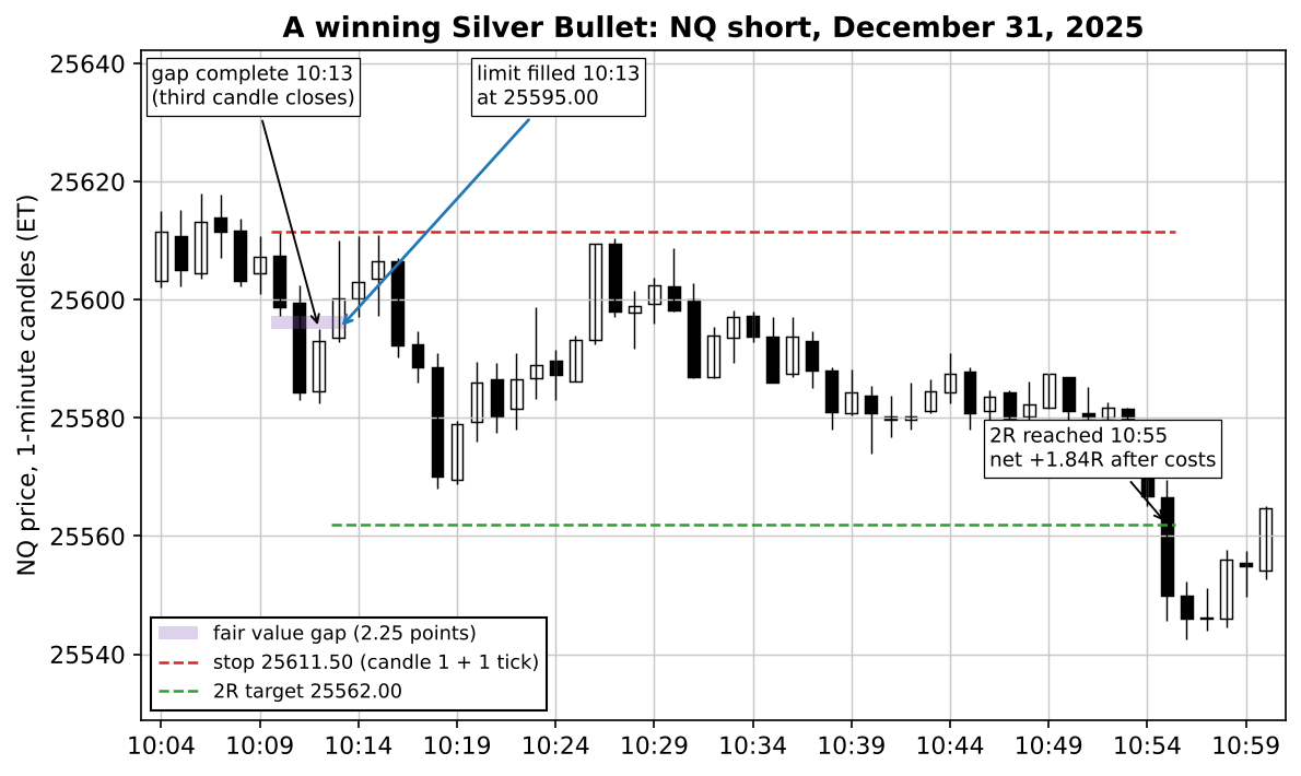
One-minute candlestick chart of NQ futures on December 31, 2025: a 2.25-point bearish fair value gap completes at 10:13, the short limit fills at 25595.00 the same minute, the stop sits at 25611.50 and the 2R target at 25562.00 is reached at 10:55 for a net gain of 1.84R after costs — A textbook winner, picked by a fixed rule: the most recent out-of-sample trade that reached 2R with a stop of typical size and lasted at least 10 minutes. The bearish gap (purple) completed at 10:13, the short filled at 25595.00, and price rallied most of the way back to the stop before falling to the target at 10:55. Net +1.84R, because costs took about 0.16R.

Study the stop line first. At 10:27 price came within one point of it before the trade worked, which is what many of these trades feel like from the inside. Then look at the last number in the caption. The stop here was 16.5 points, and the 0.01% round trip at that price is worth about 0.16R. That small fraction is where this article ends up, but the win rate comes first.

The win rate lands almost exactly on the break-even line

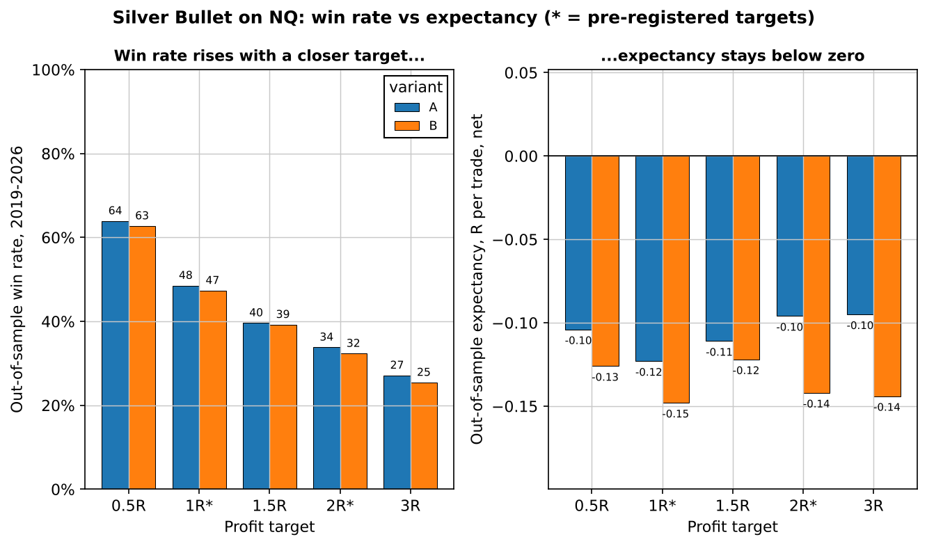
A 2R target needs to win 33.3% of the time to break even before costs, and a 1R target needs 50.0%. That's just arithmetic: one 2R winner pays for two 1R losers. So the win rate on its own says almost nothing. It has to be read next to the payoff, and the cleanest way to see that is to move the target and watch both numbers:

Two bar charts of out-of-sample results 2019-2026 for the mechanical Silver Bullet on NQ at targets of 0.5R, 1R, 1.5R, 2R and 3R: the win rate falls from 64% at 0.5R to 27% at 3R for variant A, while the net expectancy stays between -0.09R and -0.15R per trade at every target for both variants — Out-of-sample win rate (left) and expectancy after costs (right) at five targets. Only 1R and 2R were pre-registered; 0.5R, 1.5R and 3R were explored after the fact, only to show the pattern. A closer target buys a higher win rate and the expectancy doesn't move above zero at any of them.

Target	Win rate needed (before costs)	A: win rate, OOS	A: expectancy, OOS	B: win rate, OOS	B: expectancy, OOS
0.5R (explored)	66.7%	63.9%	-0.104R	62.7%	-0.126R
1R	50.0%	48.5%	-0.123R	47.3%	-0.148R
1.5R (explored)	40.0%	39.6%	-0.111R	39.2%	-0.122R
2R	33.3%	33.8%	-0.096R	32.3%	-0.142R
3R (explored)	25.0%	27.1%	-0.095R	25.4%	-0.144R

Read across any row and the pattern is the same: the win rate sits within a few points of the break-even line, on one side or the other, and the expectancy after costs is a loss of a tenth of R or more. If you set a 0.5R target, 63.9% of trades win, a number that would look great in a screenshot, and you still lose 0.104R per trade. Even at 3R, where the win rate beats its break-even line by two points, costs take it below zero. That is the point of putting win rate and expectancy side by side. A win rate is a property of where you put the target. An edge is what is left after the target, the losers and the costs. The obvious next question is how much of that loss is costs and how much is the signal.

Before costs it is zero; after costs it bleeds

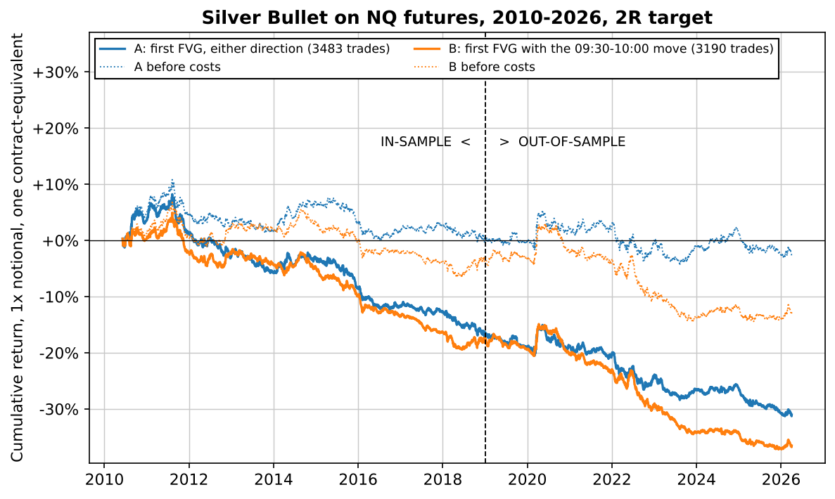
Cumulative return of the mechanical ICT Silver Bullet on NQ futures 2010-2026 at 1x notional with a 2R target: before costs variant A ends near -2% after drifting around zero, after 0.01% costs it falls steadily to -31.0%, and variant B falls to -36.5%, with no change in the trend at the 2019 out-of-sample split — Cumulative return at 1x notional (one contract's worth of exposure, no leverage), net of costs as solid lines, before costs dotted. Before costs, variant A wanders around zero for 16 years and ends at -2.3%. Costs turn that into a steady slope down to -31.0%. B is negative even before costs (-12.7%).

There is no in-sample hill and out-of-sample cliff here, which is the usual shape of an overfitted backtest. This one is flat before costs from start to finish, and costs tilt it down. The numbers in the two halves are close to each other:

2R target, net of 0.01%	A in-sample 2010–2018	A out-of-sample 2019–2026	B in-sample	B out-of-sample
Trades	1,853	1,630	1,619	1,571
Win rate	34.4%	33.8%	34.3%	32.3%
Expectancy, R per trade	-0.078	-0.096	-0.087	-0.142
Expectancy before costs	+0.016	+0.003	+0.009	-0.041
Median trade	-1.06R	-1.06R	-1.06R	-1.06R
Average trade, % of price	-0.009%	-0.012%	-0.012%	-0.017%
Profit factor	0.90	0.88	0.87	0.83
Total return, 1x notional	-16.3%	-17.6%	-17.3%	-23.3%
CAGR	-2.05%	-2.64%	-2.20%	-3.59%
Max drawdown	-23.5%	-19.1%	-23.2%	-26.2%
Time in market (of the 09:30–16:00 session)	4.29%	2.96%	3.57%	2.79%
Sharpe (daily, annualised)	-0.70	-0.76	-0.82	-1.11

The median trade is -1.06R in every column: the typical Silver Bullet trade is a full stop plus costs. About two in three trades (65.2% for A over the whole period) ended at the stop, 32.5% at the target and the rest at noon. The profit factor, total money won divided by total money lost, stayed below 1 in both halves, and the Sharpe ratio is negative in all four columns. Over the full period A lost 31.0% at 1x notional with a 36.5% drawdown. With the leverage futures traders normally use, those percentages would be several times larger. So the signal is flat and costs are what make it lose. But 0.01% sounds tiny, which is why the next section matters.

Costs eat a tenth of R on every trade

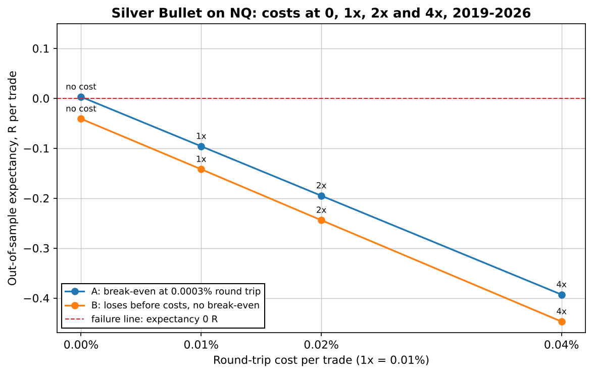
Line chart of out-of-sample expectancy in R per trade for the mechanical Silver Bullet on NQ at round-trip costs of 0, 0.01%, 0.02% and 0.04%: variant A goes from +0.003R with no costs to -0.096R, -0.195R and -0.393R, variant B from -0.041R to -0.447R, both below the zero failure line at every real cost — Out-of-sample expectancy at zero, 1x, 2x and 4x our 0.01% round trip. A only breaks even at a cost of 0.0003% of price, a fraction of a tick. B loses money before any cost is charged, so it has no break-even at all.

The problem is the size of the stop. A Silver Bullet stop sits just beyond a one-minute candle, and over the whole test the median stop was only 0.116% of price. A cost of 0.01% of price is therefore close to a tenth of the risk. Measured trade by trade, costs took 0.096R from the average variant A trade, almost exactly the difference between zero and the net result. On NQ at 23,883, the last trade in the data, 0.01% is 2.39 points; back in 2010, at 1,837, it was 0.18 points. Our cost level is meant to be conservative, but that doesn't rescue anything here: over the full period, variant A covers costs only up to 0.001% of price, which at the last price in the data is 0.24 points, less than one tick (0.25). A single tick of slippage would already cost more than that. At 2x our cost level, A loses 0.195R per trade out of sample, and at 4x, 0.393R.

I also checked the one fill assumption that flatters a limit-order strategy. My registered rule fills the limit as soon as price touches it. In real markets a touch often doesn't fill you, because others were in the queue first. Explored after the fact: requiring price to trade one tick through the limit makes it worse, not better. Variant A drops to -0.116R out of sample, B to -0.162R. The registered results above are the generous version. So costs explain the loss, but they don't explain why variant B, the "smarter" one, lost even before them.

Trading with the morning's direction made it worse

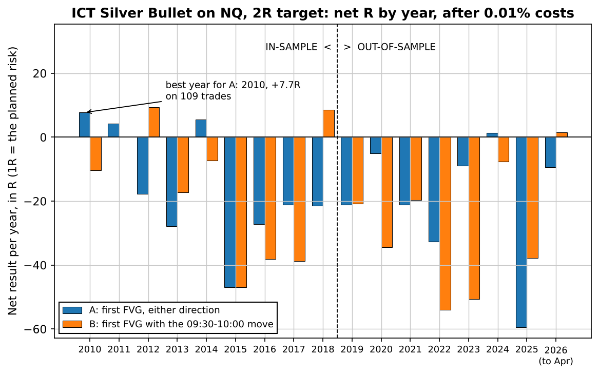
Variant B only takes gaps that point the same way as the move from the 09:30 open to 10:00. The theory is sensible: trade with the morning's order flow, not against it. In-sample it was close to A (-0.087R against -0.078R per trade). Out of sample it was clearly worse: -0.142R after costs and -0.041R before them, where A was at zero. The year-by-year record shows it wasn't one bad stretch:

Year	A trades	A net R	A win rate	B trades	B net R
2010 (from June)	109	+7.7	40.4%	95	-10.4
2011	216	+4.2	36.6%	179	+0.1
2012	207	-17.8	33.3%	181	+9.3
2013	217	-27.9	33.2%	178	-17.2
2014	220	+5.5	38.2%	181	-7.3
2015	226	-47.0	29.6%	208	-46.9
2016	220	-27.2	33.6%	197	-38.2
2017	212	-21.1	34.4%	182	-38.7
2018	226	-21.5	33.6%	218	+8.6
2019	226	-21.1	34.5%	216	-20.8
2020	228	-5.0	35.5%	220	-34.4
2021	225	-21.2	35.1%	215	-19.6
2022	216	-32.7	30.6%	214	-54.1
2023	224	-9.0	35.3%	214	-50.6
2024	228	+1.4	37.7%	222	-7.6
2025	222	-59.4	28.4%	214	-37.8
2026 (to April)	61	-9.4	31.1%	56	+1.5

Look at 2025 first. Variant A had its worst year, -59.4R, and the win rate fell to 28.4%. With a 2R target, a few points of win rate below 33.3% is the difference between a flat year and a painful one. After costs, A had 4 positive years out of 17 and B also 4. Before costs, A was positive in 9 of 17 years and B in 8: again, a coin. One caution when you compare this table with the equity chart: R weights every trade by its own stop, while the equity curve is 1x notional, so trades with small stops count for more in R, and a year can be positive in one and negative in the other. I don't have a good story for why the direction filter hurts, and I'm not going to invent one. One reading is that by 10:00 the opening move has often run its course, so a gap in its direction is late. That is a hypothesis for another test, not a finding of this one. What I can say is what this test covers and what it doesn't.

What this test says about ICT, and what it doesn't

This tests one mechanical reading of the Silver Bullet: the first gap, a fixed 1-point minimum, a stop beyond the first candle, a 2R target and nothing else. It does not test the parts of ICT that are judgement. A discretionary trader picks which gap matters, uses higher-timeframe context, and targets a specific liquidity level rather than a fixed multiple of the stop. None of that is in this code, and a skilled trader may well be adding something real. What the test does show is narrower and, I think, more useful: the raw pattern, a fair value gap in that hour, carries no edge on its own on the Nasdaq. Before costs the first gap of the window was a coin flip over 3,483 trades, and filtering by the morning's direction didn't help. If there is an edge in the Silver Bullet, it is in the trader's choices, not in the gap.

It also says something about how to read anyone's win rate. A third of trades winning at 2R, or half at 1R, is the break-even rate for those payoffs, roughly what a random entry would give in a market with no drift. Before a win rate means anything you need the payoff, the costs in R, and a sample that runs through more than one kind of market. What would change my mind is a precise rule for choosing the liquidity target that holds up out of sample after real costs, tested the same way. For a wider look at why good-looking backtests break, see why backtests fail.

Lab notes

This test was registered on 2026-10-15: rules, both variants, split, costs and the failure line, committed before a single trade was simulated. The run itself started at 03:45 UTC on October 23. My first pass put the window one minute late. I had counted the 10:00 candle as the first one, but the brief says the third candle must close between 10:00 and 10:59, and our data stamps each one-minute bar at its open, so the bar stamped 09:59 is the one that closes at 10:00. Fixing it moved the expectancy in the second decimal and the verdict not at all. Then, before writing the code for the PDF, I ran the standalone strategy.py on 2024 to 2026 and compared it with the main script: 511 trades for A and 492 for B in both, with the same expectancy to the third decimal. The surprise of the night was variant B. I expected the direction filter to be the version that worked, if any did.

So, what is the ICT Silver Bullet win rate? About a third at 2R, about half at 1R, and neither is an edge once you count the losers and the costs. The pattern turns up almost every morning. On its own, it doesn't pay.

Get the Silver Bullet rules + the Python code (PDF)

Every rule from this test on one page, the results table, and standalone Python you can run on your own data. Free, by email.

Instant delivery. One PDF, no spam. Unsubscribe anytime.

FAQ

What is the ICT Silver Bullet strategy?

It is an intraday setup taught publicly by The Inner Circle Trader (Michael J. Huddleston): during the 10:00 to 11:00 New York window, wait for a fair value gap, a three-candle pattern where the third candle's low is above the first candle's high (or the mirror for shorts), enter when price comes back into the gap, and aim for the next pool of liquidity. Our test used a mechanical reading of it: the first gap of at least 1 point, a limit order at the gap edge, a stop beyond the first candle and a 2R target.

What is the ICT Silver Bullet win rate?

In our mechanical test on NQ futures from 2010 to 2026, it won 34.1% of 3,483 trades with a 2R target and 49.5% with a 1R target. Out of sample (2019 to 2026) the figures were 33.8% and 48.5%. Those are almost exactly the win rates a 2R and a 1R payoff need just to break even (33.3% and 50.0%), so after costs the expectancy was negative: -0.096R per trade out of sample.

Does the Silver Bullet strategy work?

Not as a mechanical rule in our test. Both pre-registered variants, the first fair value gap of the window and the first gap in the direction of the 09:30 to 10:00 move, had a negative out-of-sample expectancy after 0.01% round-trip costs (-0.096R and -0.142R per trade), which crosses the failure line we fixed in advance. Before costs the first variant earned +0.003R per trade, which is zero. Discretionary traders apply judgement about liquidity that this test does not capture.

Is there an ICT Silver Bullet strategy PDF?

Yes. EdgeLab's free PDF has every rule from this test on one page, the results table for both variants, and standalone Python code you can run on your own 1-minute data, with switches for the variant and the target. It is sent by email from the signup box in the article.

Backtest notice: NQ (E-mini Nasdaq-100) futures, Databento continuous one-minute data, New York time, 4,043 mornings from June 7, 2010 to April 2, 2026, 09:30 to 12:00 only. Costs modelled at 0.01% of price per round trip. Every position is closed by 12:00, so the unadjusted contract switches in the continuous series (in the evening, New York time) never fall inside a trade. In-sample to 2018-12-31, out-of-sample from 2019-01-01; Sharpe annualised from daily returns at the actual number of trading days per year; returns at 1x notional, no leverage. The Silver Bullet concept is The Inner Circle Trader's (Michael J. Huddleston); the rules tested here are EdgeLab's own mechanical reading, and the discretionary judgement of the method can't be fully captured in code. Backtested performance is hypothetical. Past performance does not guarantee future results. This is research, not financial advice.

Robin Eriksson

Founder of EdgeLab. Five years of discretionary losses taught me to test everything — now I publish the strategies that survive. About me →

ICT Silver Bullet strategy: what 16 years of Nasdaq futures say about its win rate